Why We Pay More Than We’re Likely to Lose
The Shape of the Loss
The first thing to recognize is that “expected medical spending” hides what insurance is really about. The expected value of a household’s annual medical spending is not very informative on its own, because the distribution is sharply right-skewed.
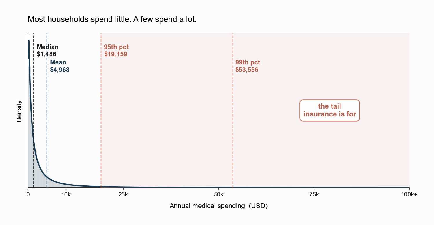
The figure shows a stylized distribution of annual medical spending. Most households cluster near the bottom: the median spending is around $1,500. But the mean is more than three times the median, because a small number of households have catastrophic years that pull the average up. The 95th percentile is around $21,000, and the 99th is around $60,000.
When we say “expected loss,” we are referring to the mean of this distribution. Risk-neutral pricing would set the premium equal to that mean. But what people actually care about, when they buy insurance, is not the mean. It is the spread between the typical year and the catastrophic one. The reason a $24,000 family premium feels reasonable is that it converts a lottery in which most outcomes are mild but a few are devastating into a flat payment.
The Expected-Utility Framework
Let a worker enter the period with initial wealth \(w_0\) and face a random monetary loss \(\tilde{L} \ge 0\) (for instance, out-of-pocket medical spending). Final wealth without insurance is \[ \tilde{W} = w_0 - \tilde{L}. \]
Under the von Neumann-Morgenstern axioms, the worker has a continuous utility function \(u(\cdot)\) over wealth, and ranks risky prospects by their expected utility \[ EU = E\!\left[u(\tilde{W})\right] = \int u(w_0 - L)\,dF(L), \] where \(F\) is the cumulative distribution of \(\tilde{L}\). Two wealth distributions are ranked by their expected utilities, not by their expected values. This single shift, from \(E[\tilde{W}]\) to \(E[u(\tilde{W})]\), is the entire conceptual machinery we need to motivate the demand for insurance.
The shape of \(u\) is what distinguishes a risk-averse worker from a risk-neutral one.
- Risk neutral: \(u\) is linear. The worker cares only about \(E[\tilde{W}]\) and is unwilling to pay anything above the expected loss.
- Risk averse: \(u\) is strictly concave, \(u''(w) < 0\). The worker cares about both the mean and the dispersion of \(\tilde{W}\), and is willing to pay a strictly positive premium to reduce dispersion.
- Risk loving: \(u\) is convex. The worker would pay to increase risk, and would never buy insurance.
What does it mean for \(u\) to be concave? In everyday terms, it means each additional dollar matters a little less than the one before it. The first $10,000 of annual income makes a huge difference to a household’s living standards. The hundredth $10,000 matters much less. This is what economists call diminishing marginal utility of wealth. It is the workhorse assumption for almost everything that follows, and it matches what most people would say if you asked them to compare the value of $10,000 in a comfortable year versus $10,000 in a year when they are scrambling to cover a hospital bill.
Jensen’s Inequality and the Geometry of Risk
The mathematical reason a risk-averse worker pays for insurance is Jensen’s inequality. For any strictly concave \(u\) and any non-degenerate lottery \(\tilde{W}\), \[ E\!\left[u(\tilde{W})\right] \;<\; u\!\left(E[\tilde{W}]\right). \] The expected utility of a risky payoff is strictly less than the utility of the expected payoff. Geometrically, the chord connecting two points on a concave curve lies below the curve itself.
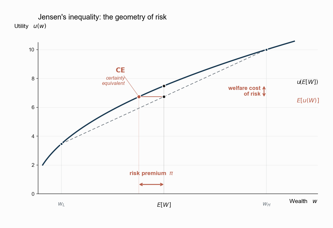
The figure makes the geometry concrete with a two-state lottery: wealth \(w_L\) with probability \(p\) and \(w_H\) with probability \(1-p\).
- The point \(u(E[\tilde{W}])\) on the curve gives the utility a worker would attain with certainty at the mean wealth.
- The point \(E[u(\tilde{W})]\) on the chord gives the utility a worker actually attains with the lottery.
- The vertical gap between the two is the welfare cost of risk. Eliminating it is what insurance does.
The horizontal distance is the dollar version of the same idea. Define the certainty equivalent \(CE\) implicitly by \[ u(CE) \;=\; E\!\left[u(\tilde{W})\right]. \] \(CE\) is the certain wealth a worker would accept in lieu of the lottery. Because \(u\) is concave, \(CE < E[\tilde{W}]\). The risk premium is the dollar gap: \[ \pi \;\equiv\; E[\tilde{W}] - CE \;>\; 0. \] This is the maximum amount the worker would pay, above and beyond the expected loss, to convert the lottery \(\tilde{W}\) into its mean for certain.
A risk-neutral observer looks at insurance and sees a negative-NPV transaction. A risk-averse worker looks at the same transaction and sees a wealth distribution with the same mean but no variance, and is willing to pay \(\pi\) for the swap. The “irrational” extra payment is the price of removing variance.
Putting numbers on it. Suppose a household has $80,000 in wealth at the start of the year, with a 5% chance of a $60,000 loss and a 95% chance of zero loss. The expected loss is $3,000. The expected wealth is $77,000. But the certainty equivalent (the certain wealth that gives the same utility as the lottery) might be only $75,000 under reasonable risk aversion. The risk premium is then $2,000, on top of the $3,000 expected loss. A premium of $5,000 would make this household exactly indifferent between buying full insurance and going without. Anything below $5,000 is a strict gain.
The Pratt-Arrow Approximation
How big is \(\pi\)? For small risks, a second-order Taylor expansion gives a clean answer.
Let the loss be \(\tilde{L} = E[\tilde{L}] + \tilde{\varepsilon}\) where \(\tilde{\varepsilon}\) is a mean-zero shock with variance \(\sigma^2\). Write final wealth as \(\tilde{W} = \bar{w} - \tilde{\varepsilon}\) with \(\bar{w} = w_0 - E[\tilde{L}]\). Expand \(u(\bar{w} - \tilde{\varepsilon})\) around \(\bar{w}\): \[ u(\bar{w} - \tilde{\varepsilon}) \;\approx\; u(\bar{w}) - u'(\bar{w})\,\tilde{\varepsilon} \,+\, \tfrac{1}{2}\,u''(\bar{w})\,\tilde{\varepsilon}^2. \] Taking expectations and using \(E[\tilde{\varepsilon}]=0\), \(E[\tilde{\varepsilon}^2]=\sigma^2\), \[ E[u(\tilde{W})] \;\approx\; u(\bar{w}) + \tfrac{1}{2}\,u''(\bar{w})\,\sigma^2. \] Setting \(u(\bar{w} - \pi) = E[u(\tilde{W})]\) and expanding the left side to first order yields \[ u(\bar{w}) - u'(\bar{w})\,\pi \;\approx\; u(\bar{w}) + \tfrac{1}{2}\,u''(\bar{w})\,\sigma^2, \] and therefore \[ \boxed{\;\pi \;\approx\; \tfrac{1}{2}\,\sigma^2\,A(\bar{w}),\quad\text{where}\quad A(w) \;\equiv\; -\frac{u''(w)}{u'(w)}.\;} \]
This is the Pratt (1964) and Arrow (1971) approximation. It says the risk premium is, to a second-order approximation, the product of two objects:
- \(\sigma^2\), the variance of the loss. Bigger losses raise the price of bearing the risk.
- \(A(w)\), the coefficient of absolute risk aversion, which measures the local curvature of \(u\) relative to its slope. A more concave utility implies a larger premium for the same variance.
Two qualitative consequences follow. First, willingness to pay for insurance scales with variance, not with expected loss, which is why people insure unlikely but large losses (catastrophic medical events) more aggressively than likely but small ones (a prescription copay). Stated another way, two health risks with the same expected dollar loss have very different insurance value if one is “lose $1,000 every year” and the other is “lose $0 most years, but $1 million once a decade.” The second one is what people are really afraid of. Second, if \(A(w)\) falls with wealth (decreasing absolute risk aversion), wealthier households should be relatively less interested in insurance against the same risk. A comparative-static prediction one can take to the data.
Arrow’s Demand for Insurance
Pratt-Arrow tells us what the risk is worth. Arrow (1963), in his foundational paper on the welfare economics of medical care, asks the next question: what shape of contract optimally absorbs that risk?
Consider an indemnity contract that pays the worker \(I(L)\) when the realized loss is \(L\), in exchange for a premium \(P\) paid up front. Final wealth becomes \[ \tilde{W} \;=\; w_0 - P - \tilde{L} + I(\tilde{L}). \] The insurer earns expected profit \[ \Pi \;=\; P - (1+\lambda)\,E[I(\tilde{L})], \] where \(\lambda \ge 0\) is the proportional load factor that accounts for administrative costs and the insurer’s risk-adjusted required return.
Arrow’s theorem (full insurance under fair pricing). If insurance is actuarially fair, \(\lambda = 0\), then the worker’s optimal contract is full insurance: \(I(L) = L\) for all \(L\). The reasoning is exactly Jensen’s inequality. Under \(\lambda = 0\) the worker can convert the lottery into its mean at zero cost. Any contract that leaves residual risk on the worker is strictly dominated by one that eliminates that residual risk.
Arrow’s theorem (deductible under loaded pricing). When \(\lambda > 0\), full insurance is no longer optimal. Arrow showed that the optimal contract has the form \[ I^*(L) \;=\; \max\{\,L - D,\; 0\,\}, \] that is, a deductible \(D > 0\), with full coverage of losses above \(D\). The intuition is the same one that drives every real-world health plan with a deductible. The load makes coverage of small losses too expensive relative to the risk-protection value they provide. The contract concentrates coverage on the part of the distribution where the risk premium per dollar of variance is largest, namely the tails. This is exactly why most U.S. health plans have a deductible: you pay for routine doctor visits and prescriptions out of pocket, but once your costs cross a threshold (often $2,000 or $3,000), the plan starts paying. The optimum is to insure the tail, not the body, of the distribution.
Mossin’s coinsurance theorem (Mossin, 1968). If the contract is restricted to proportional coverage \(I(L) = \alpha L\) for some \(\alpha \in [0, 1]\), the optimal \(\alpha\) is strictly less than one whenever \(\lambda > 0\). The worker rationally chooses to bear some of the loss because the marginal load on the last dollar of coverage exceeds its marginal risk-protection value.
Arrow’s two results say: with fair pricing, the optimal contract removes all risk; with loaded pricing, the optimal contract removes only the part of risk that is most expensive to bear. Both follow from the same machinery, namely the curvature of \(u\), but only the second one is what real markets implement.
What This Framework Cannot Yet Explain
Everything above assumes that the insurer and the worker share the same distribution \(F\) over \(\tilde{L}\). The premium \(P\) is then a price for the physical risk, and the only question is how much of it the worker wants to offload.
Real insurance markets do not work this way. The worker often knows things about \(\tilde{L}\) that the insurer does not: a chronic condition, a family history, a planned procedure. Imagine two thirty-five-year-olds applying for the same policy. One is a marathon runner with no family history of disease. The other has Type 1 diabetes and a parent who had cancer at fifty. They look identical on the application form, but they are not the same risk. Once the two sides of the contract have different beliefs about the same loss, the premium is no longer a clean price for risk-bearing. It becomes a price that selects who buys at all, and at that point the entire equilibrium structure derived from Arrow’s theorem can collapse.
That collapse is the subject of the next note. The Pratt-Arrow machinery survives. What fails is the assumption that the insurer can write a contract whose price reflects the average loss, when the average depends on who self-selects into the pool.
References
Arrow, K. J. (1963). Uncertainty and the Welfare Economics of Medical Care. American Economic Review, 53(5), 941–973.
Arrow, K. J. (1971). Essays in the Theory of Risk-Bearing. Markham Publishing.
Mossin, J. (1968). Aspects of Rational Insurance Purchasing. Journal of Political Economy, 76(4), 553–568.
Pratt, J. W. (1964). Risk Aversion in the Small and in the Large. Econometrica, 32(1/2), 122–136.