When Raising the Price Raises the Cost
A Market in Which Cost Depends on Price
In every textbook supply-and-demand diagram, the cost of producing the marginal unit is a property of the seller’s technology. Doubling the price brings in more producers willing to supply at the higher price, but the cost of making any individual unit does not depend on what price the firm charges.
Insurance markets break this assumption in an essential way. The cost of producing the marginal contract is a property of the buyer who chooses to purchase at that price. When asymmetric information lets buyers select into the contract on the basis of their own risk, raising the price drives away the cheapest buyers first and leaves the insurer with a costlier pool. Cost depends on price.
To see what that means concretely, suppose a health insurer raises its monthly premium from $400 to $500. In a textbook market, the only effect is that some buyers no longer think coverage is worth the price and stop buying. The remaining buyers are just a smaller version of the same pool, and the cost of insuring them is unchanged. In an insurance market, the buyers who drop out at the higher price are the healthiest ones, the people who were on the margin because their expected claims were lowest. The buyers who stay are sicker on average. The insurer’s per-buyer cost has risen, even though the contract itself has not changed.
This is the conceptual contribution of Einav, Finkelstein, and Cullen (2010), hereafter EFC. Their framework takes the Rothschild-Stiglitz primitives from Health Insurance 2 and re-draws them as a demand curve, an average-cost curve, and a marginal-cost curve. Once the diagram is built, all the standard welfare machinery of textbook microeconomics applies. The triangle of deadweight loss can be read off the picture, and the price of identifying it falls out of how much variation in \(P\) one observes in the data.
Setting Up the Diagram
Fix a single insurance contract, say, a generous health plan with a defined benefit package. Let the quantity \(Q \in [0, 1]\) be the fraction of a target population that purchases this contract at a given price \(P\).
Inverse demand \(D(Q)\). Let workers be heterogeneous in their willingness to pay for coverage. Order them from highest to lowest willingness to pay. The inverse demand \(D(Q)\) is the willingness to pay of the \(Q\)-th worker, that is, of the marginal buyer when the quantity sold is \(Q\). By construction, \(D\) is downward sloping.
Marginal cost \(MC(Q)\). Let \(c_i\) be the expected loss the insurer incurs if it insures worker \(i\) under this contract. The marginal cost curve \(MC(Q)\) is the expected cost the insurer faces from insuring the \(Q\)-th worker, namely the worker who is just on the margin of buying at the corresponding price. Crucially, \(MC\) depends on the identity of the marginal buyer, not on the insurer’s production technology.
Average cost \(AC(Q)\). The average cost curve is the average \(c_i\) across all \(Q\) workers in the pool when the quantity sold is \(Q\), \[ AC(Q) \;=\; \frac{1}{Q}\int_0^{Q} MC(s)\, ds. \] If \(MC\) is monotone, \(AC\) inherits the same monotonicity but with smaller magnitude per unit of \(Q\).
The sign of the relationship between willingness to pay and expected cost is what distinguishes adverse selection from advantageous selection.
- Adverse selection. Workers with the highest willingness to pay also have the highest expected loss. Sicker workers value coverage more and cost more. Ordering buyers by willingness to pay therefore orders them by cost, in the same direction. \(MC(Q)\) is downward sloping, and \(AC(Q)\) lies above \(MC(Q)\) everywhere.
- Advantageous selection. Workers with the highest willingness to pay have lower expected loss. This sounds paradoxical, but it arises naturally when willingness to pay is driven by traits like risk aversion, income, and health-consciousness that are negatively correlated with claims cost. \(MC\) slopes upward and \(AC\) lies below \(MC\).
Adverse Selection in the EFC Diagram
The figure below shows the textbook adverse-selection case. Demand \(D(Q)\) slopes down (more workers buy at lower prices), \(MC(Q)\) slopes down (the marginal buyer at higher \(Q\) is healthier and cheaper), and \(AC(Q)\) lies above \(MC(Q)\).
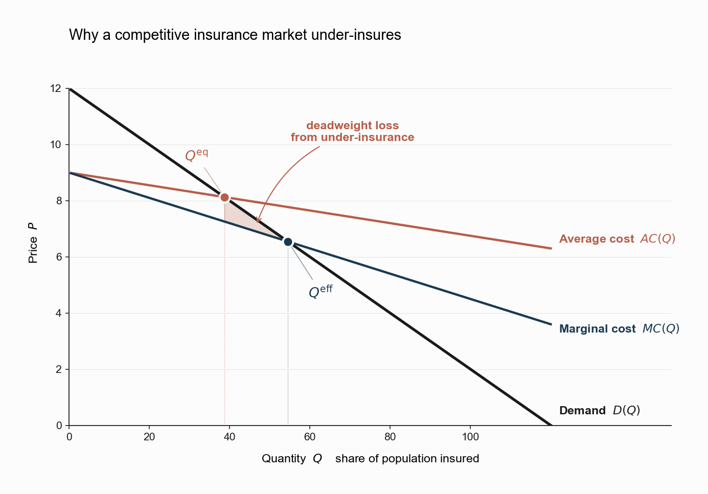
Two equilibrium quantities sit on the diagram.
- Competitive equilibrium \(Q^{\rm eq}\). A competitive insurer must break even on the pool it actually serves. The zero-profit condition is \(P = AC(Q)\). Demand intersects \(AC\) at \(Q^{\rm eq}\). Every worker to the left of \(Q^{\rm eq}\) is willing to pay at least the average cost of the pool of buyers, and is insured.
- Efficient quantity \(Q^{\rm eff}\). From a social planner’s perspective, the marginal contract should be sold to a worker iff their willingness to pay exceeds the cost the planner incurs by adding that worker to the pool, that is, \(D(Q) \ge MC(Q)\). Demand intersects \(MC\) at \(Q^{\rm eff}\).
Under adverse selection, \(MC < AC\) over the relevant range and therefore \(Q^{\rm eq} < Q^{\rm eff}\). The competitive market under-provides coverage. Workers in the interval \([Q^{\rm eq}, Q^{\rm eff}]\) have willingness to pay above their own marginal cost but below the average cost of the existing pool, so they are not insured even though insuring them would be welfare-improving.
The deadweight loss triangle is the shaded region in the figure, with area \[ DWL \;=\; \int_{Q^{\rm eq}}^{Q^{\rm eff}} \big[\,D(Q) \;-\; MC(Q)\,\big]\,dQ. \]
The geometry has a sharp economic interpretation. The cause of the welfare loss is not that some workers are uninsured. It is that the workers whose own cost would justify their coverage are nonetheless not insured, because they cannot avoid being grouped with sicker, costlier buyers in the competitive pool.
Walking through with the kitchen-table analogy: imagine a young, healthy worker whose own expected medical spending is $2,000 a year. She would happily buy a plan for $3,000. But the pool of people who buy this plan has an average cost of $5,000, because it includes a lot of sicker people. So the insurer has to charge $5,000 to break even. She drops out, even though it would have been welfare-improving for the insurer to take her at $3,000. The reason it could not is that taking her at $3,000 would have meant taking the sicker buyers at $3,000 too, and that would have lost money. The market cannot separate her from them, and so it loses her altogether.
EFC’s empirical insight is that all three curves can be estimated from price variation. If a researcher observes a shift in the price of a given contract, whether through a policy reform, a subsidy change, or some other exogenous variation, and tracks the resulting change in \(Q\) and the resulting change in average claims per insured worker, one obtains points along \(D\) and along \(AC\). Differentiating \(Q \cdot AC(Q)\) with respect to \(Q\) recovers \(MC\). The welfare triangle is then a quantity one can numerically compute, not merely qualitatively assert.
Advantageous Selection and Its Mirror Geometry
The opposite case is far from a textbook curiosity. Empirically, Finkelstein and McGarry (2006) found advantageous selection in the long-term care insurance market: buyers were less likely to enter a nursing home than non-buyers. The mechanism is that risk aversion and prudence drive both insurance purchase and preventive behavior, and the latter reduces claims.
The intuition is not as paradoxical as it sounds. The kind of person who buys long-term care insurance years before they might need it is the kind of person who also exercises, has annual physicals, takes their medications, and plans ahead in general. All of those behaviors also reduce the probability they end up in a nursing home. The buyers of the policy are therefore healthier than the non-buyers, on the margin that matters for claims.
In an advantageously selected market, \(MC\) slopes upward (the marginal buyer at higher \(Q\) is sicker and costlier than the inframarginal one) and \(AC\) lies below \(MC\). The competitive equilibrium \(Q^{\rm eq}\) now lies above \(Q^{\rm eff}\): the market over-insures. Workers who would not be willing to pay their own marginal cost are nonetheless drawn into the pool because the average cost they would pay is lower than the marginal cost they would impose.
The welfare loss is again a triangle, but on the other side of \(Q^{\rm eff}\) and bounded above by \(MC\) rather than below by it. The policy implication is also inverted. Under adverse selection, mandates and subsidies that pull more buyers into the pool improve welfare. Under advantageous selection, those same instruments worsen welfare.
The sign of the slope of \(MC\) is therefore a first-order policy parameter. EFC’s framework makes the case that estimating it is, in many selection markets, more useful than estimating any structural primitive of the underlying R-S model. If you do not know whether a market is adversely or advantageously selected, you do not even know whether a subsidy is welfare-improving or welfare-destroying.
What This Framework Does and Does Not Identify
EFC’s framework is powerful because it reduces a high-dimensional information problem to a three-curve diagram. But the price of that reduction is two pieces of structure that it deliberately suppresses.
It does not identify moral hazard. The cost curves \(MC\) and \(AC\) are estimated from realized claims among insured workers. If insurance itself changes claims behavior, through an ex-ante or ex-post moral-hazard channel, then the cost a worker imposes on the insurer when insured is not the same as the loss they would experience uninsured. The EFC welfare triangle conflates the two unless one has an independent way to separate selection from moral hazard. That separation problem is the subject of the next note.
It does not identify the source of selection. EFC’s \(MC\) tells us how much cheaper the marginal buyer is relative to the inframarginal one, but not why. The price elasticity of selection captures the joint distribution of willingness to pay and expected cost. It does not say whether the underlying heterogeneity is in private information about health, in risk aversion, in income, or in something else entirely. Hackmann, Kolstad, and Kowalski (2015) and Mahoney and Weyl (2017) extend the diagram to nest these mechanisms more explicitly, but the basic EFC picture is silent on them.
These limitations are features, not bugs. EFC’s contribution is to isolate the welfare consequence of selection without committing to a specific model of why selection arises. Whatever the microfoundation, if the data show \(D\), \(MC\), and \(AC\) drifting apart in the predicted pattern, the welfare cost is there to be measured.
Looking Ahead
We have now drawn the picture of how insurance markets fail when buyers know more than sellers. But all of this analysis treated the loss distribution as a property of the worker, unaffected by the contract they hold. That assumption is the next thing to give up.
When having insurance changes the behavior that generates the loss, whether through reduced precaution, increased utilization, or anything in between, the cost of insuring the same worker depends on whether they are insured. This is moral hazard, and in Health Insurance 4 we will see how it changes both the optimal contract and the empirical identification of selection effects. The Pratt-Arrow logic for the demand for risk-bearing survives. What we will have to add is a model of how the supplier of risk-bearing also changes what they are insuring against.
References
Einav, L., Finkelstein, A., & Cullen, M. R. (2010). Estimating Welfare in Insurance Markets Using Variation in Prices. Quarterly Journal of Economics, 125(3), 877–921.
Einav, L., Finkelstein, A., & Levin, J. (2010). Beyond Testing: Empirical Models of Insurance Markets. Annual Review of Economics, 2, 311–336.
Finkelstein, A., & McGarry, K. (2006). Multiple Dimensions of Private Information: Evidence from the Long-Term Care Insurance Market. American Economic Review, 96(4), 938–958.
Hackmann, M. B., Kolstad, J. T., & Kowalski, A. E. (2015). Adverse Selection and an Individual Mandate: When Theory Meets Practice. American Economic Review, 105(3), 1030–1066.
Mahoney, N., & Weyl, E. G. (2017). Imperfect Competition in Selection Markets. Review of Economics and Statistics, 99(4), 637–651.