How Do You Measure a Job Change That Did Not Happen?
The Counterfactual Problem
Job Lock 1 developed an explicit model of how employer-sponsored insurance distorts the outside option in a search environment. The model produced three sharp comparative-static predictions about mobility, wage gains, and match quality. We did not, however, say anything about how to test those predictions in real data.
The reason this is hard is structural, not a question of data availability. Job lock is, in essence, the absence of a move that would otherwise have happened. Researchers observe the moves that did occur, the workers who stayed, the wages of each. What they do not observe, and cannot directly measure, is the counterfactual world in which the lock did not bind. Estimating the magnitude of the lock therefore requires variation that selectively relaxes the wedge for some workers and not others, in a way uncorrelated with those workers’ underlying mobility preferences.
To get a feel for what successful identification looks like at the population level, consider the picture of who moves where as workers change jobs.
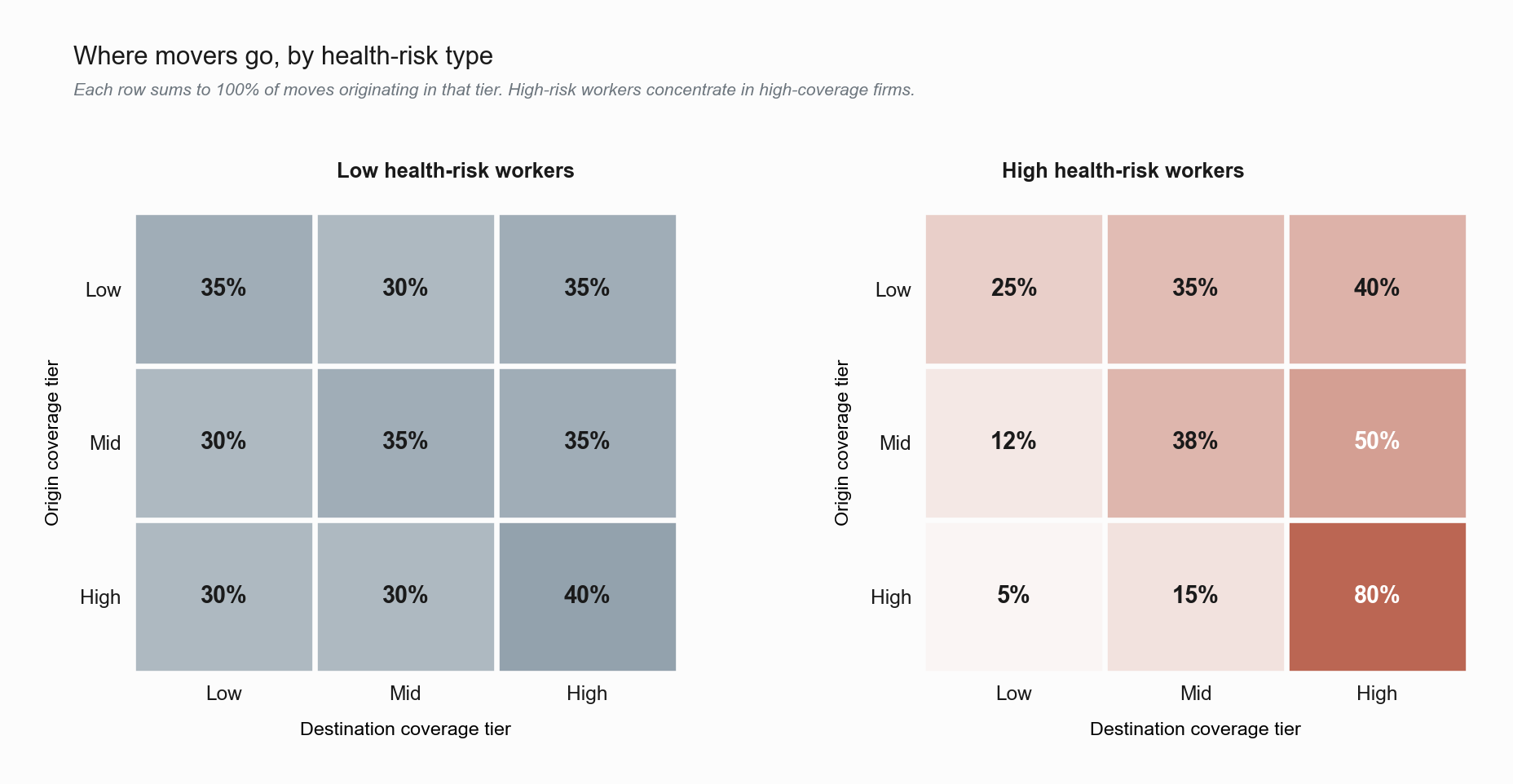
The two panels show stylized mover transition matrices in a Card-style cross-tabulation. Rows are the worker’s origin coverage tier (low / mid / high) and columns are the destination, so each row sums to 100% of moves originating in that tier. The left panel is low health-risk workers. Their moves spread roughly evenly across destination tiers, because the coverage margin is not the binding consideration in their decision. The right panel is high health-risk workers. The mass concentrates in the rightmost column: 40% of low-tier movers, 50% of mid-tier movers, and 80% of high-tier movers land at high-coverage firms. The lower triangle (moving down a tier) almost empties out. The heatmap makes the sorting visible in a way that a single event-study coefficient cannot. The high-\(h\) panel is what the comparative statics of Job Lock 1 predict: the acceptance set has expanded toward coverage-preserving firms and shrunk away from coverage-losing ones.
All figures in this note are stylized illustrations. The numbers are simulated, not estimated. The point is to fix what the design looks like when it works.
This note surveys the four most credible sources of variation in the U.S. context, the canonical estimating equation, and the reasons no single source can answer the full question on its own.
Four Sources of Identifying Variation
Recall from Job Lock 1 that the lock wedge is \[
w_{\text{lock}}(h) \;=\; \min\big\{\,\bar{p}(h) - v(h),\;\; \pi(h)\,\big\},
\] the per-period cost a worker incurs by losing the firm pool. Any source of variation that exogenously shrinks this wedge for some workers and not others identifies the labor-market consequence of the wedge. The four leading sources in the literature are.
Spousal coverage. A married worker whose spouse has independent ESI through a different employer faces a much smaller \(w_{\text{lock}}(h)\). If the worker separates, the spouse’s plan can cover them. Conditional on health type \(h\), having a spouse with portable coverage is the closest empirical analogue to a no-wedge counterfactual. Madrian (1994) and many follow-up papers exploit this variation, comparing mobility of workers with versus without alternative coverage.
Imagine two Marias from Job Lock 1. One is married to a teacher with a generous union health plan. The other is a single parent. Their health risks are the same. Their jobs are the same. Their decisions about whether to leave their employer should not be the same, because the second Maria’s wedge is much larger. The difference in their mobility rates is the part attributable to ESI dependence.
Medicare eligibility at age 65. When a worker turns 65, they automatically gain access to Medicare, which is fully portable. The wedge effectively vanishes at the eligibility threshold. The discontinuity allows a regression-discontinuity design centered on the worker’s 65th birthday. This is the variation exploited by, among others, Gustman and Steinmeier (1994) and more recently by Strumpf (2010) in the context of retirement timing.
Public-insurance expansions. State-level Medicaid expansions before the ACA, and the federal ACA Medicaid expansion of 2014, increased the availability of subsidized non-employer coverage for low-income workers. The expansions varied across states and over time, generating a difference-in-differences design with state-by-time fixed effects. Hamersma and Kim (2009), Heim and Lurie (2010), and Garthwaite, Gross, and Notowidigdo (2014) all use this kind of variation.
ACA exchange marketplaces. The 2014 introduction of state and federal exchanges created, for the first time on a national scale, a subsidized individual market with community rating and a guarantee-issue requirement. For non-elderly adults above the Medicaid cutoff, this is a direct portability shock, although one whose magnitude varies with income, family structure, and state-level decisions about exchange architecture. The post-2014 literature exploits the timing and geographic variation of this rollout.
Each source has its own strengths and its own threats to identification. None of them is the “natural experiment” social scientists fantasize about. They are all DiD or RD designs that require specific parallel-trends or local-randomization assumptions to support a causal interpretation.
The Canonical Estimating Equation
Most modern job-lock studies estimate variants of an event-study regression of the form \[ y_{ist} \;=\; \sum_{k \neq -1} \beta_k \cdot \mathbf{1}\{t - t^*_s = k\} \cdot \text{Treated}_i \,+\, \alpha_i \,+\, \gamma_{st} \,+\, \varepsilon_{ist}, \] where \(y_{ist}\) is a mobility outcome for worker \(i\) in state \(s\) at time \(t\), \(t^*_s\) is the date of the relevant policy event in state \(s\) (or a worker-level age threshold), \(\text{Treated}_i\) is an indicator for a worker whose lock wedge is plausibly affected by the event (high-\(h\), no spousal coverage, low income, etc.), and the \(\beta_k\) coefficients are the dynamic event-study estimates relative to the omitted base period \(k = -1\).
The two identifying conditions are by now standard.
- Parallel pre-trends. The \(\beta_k\) for \(k < 0\) should be statistically and economically indistinguishable from zero. This says that, conditional on the controls, the treated and untreated groups were trending similarly before the event.
- No anticipation. Workers cannot adjust their behavior in anticipation of the event in a way that would contaminate the pre-period estimates. For age-based events (Medicare, dependent coverage) this is harder to defend than it sounds. Workers do know in advance when they will turn 65, and the literature has developed bias-adjusted estimators that allow for partial anticipation.
The figure below shows a stylized version of what a clean event study should look like. The pre-period \(\beta_k\) are tightly distributed around zero. At the event date the treated group’s mobility outcome begins to diverge from the control group’s, building gradually over a few years as the lock relaxes and workers re-optimize their job choices.
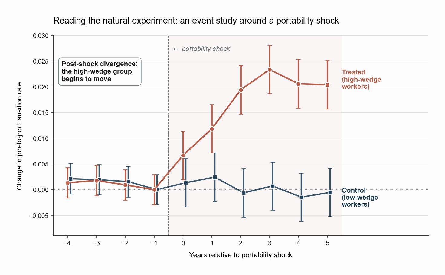
The shape of the post-period response carries information about the kind of friction the lock generates. A sharp impact effect followed by a flat plateau is consistent with a binding constraint that workers had been waiting to release. A gradual ramp is consistent with a friction in match formation, where workers re-enter the search process but only realize gains as new matches are formed over time. A delayed or absent effect is consistent with a small lock, or with an offsetting channel (e.g., the new coverage option being too expensive to be attractive in equilibrium).
This is a stylized illustration only. The numbers are simulated, and the figure should not be read as evidence about any specific policy. The point is to fix the geometry of what an event-study identification of job lock looks like when it works.
Madrian’s DiD and Its Heirs
Madrian (1994), already discussed in Job Lock 1, was the prototype. Her design compared workers with versus without spousal coverage and found mobility roughly 25 percent lower for the locked group. Subsequent literature has tested whether this finding survives more careful specification.
- Refinement of the comparison group. Sanz-de-Galdeano (2006) showed that the Madrian estimate is sensitive to how the “alternative coverage” group is defined. A naive contrast between any married worker and any unmarried worker conflates the lock with other features of marital status that affect mobility.
- Direct measurement of the wedge. Cooper and Monheit (1993) and others tried to directly measure the value workers placed on coverage, to construct a continuous measure of the wedge rather than a binary “locked vs. not” indicator. These efforts produced smaller but generally still positive estimates.
- Alternative outcomes. Some papers measure entrepreneurship rather than job-to-job moves, on the grounds that leaving to start a business is the move most directly inhibited by losing employer coverage. Fairlie, Kapur, and Gates (2011) document a large jump in self-employment at age 65 attributable to Medicare-driven portability. A concrete reading: an aspiring entrepreneur cannot afford to walk away from a salaried job if it is also her only access to coverage. When she turns 65 and Medicare becomes available, she suddenly can. The visible spike in startup activity right at the 65 cutoff is the lock releasing.
The cumulative weight of this literature is that something is going on. The basic mechanism in Job Lock 1 is consistent with the data. But the magnitudes vary widely by design, sample, and outcome, and the variation is systematic: estimates from spousal-coverage DiDs are larger than estimates from Medicaid expansions, which are in turn larger than estimates from the post-2014 ACA studies. The forest plot below collects representative point estimates from each of the four identification families.
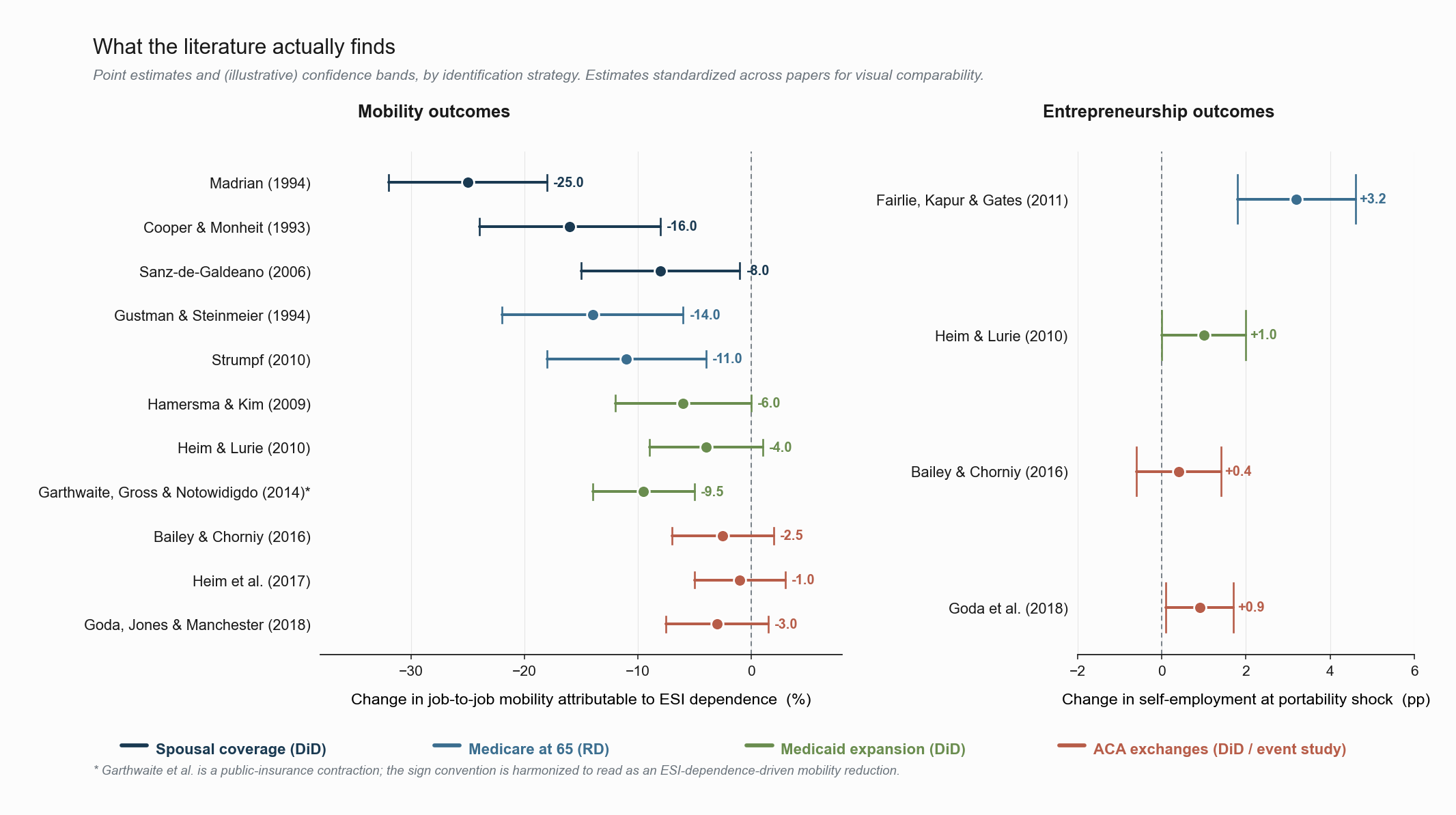
The figure has two panels. The left panel collects mobility estimates, expressed as the percentage change in job-to-job transitions attributable to ESI dependence (negative values mean the lock binds). The right panel collects the much smaller entrepreneurship literature, expressed as the percentage-point change in self-employment around a portability shock. Three patterns are visible at a glance.
First, the spousal-coverage DiD lineage (navy) delivers the largest absolute magnitudes, with Madrian’s original 25% reduction sitting at the upper end of the band. Second, the natural-experiment designs centered on age 65 (slate) and Medicaid contractions or expansions (green) cluster in the 6%–14% range, smaller than the spousal estimates but consistently signed. Third, the post-2014 ACA estimates (orange) are noisy, small, and frequently straddle zero. This is the “puzzle of small effects” that the next section takes up. The right-panel entrepreneurship results show the same ordering: the Medicare-65 RD design of Fairlie et al. delivers a sharp positive jump, the Medicaid and ACA estimates are an order of magnitude smaller.
Estimates have been standardized across papers for visual comparability and the confidence bands are illustrative of typical precision rather than exact replications. The structural fact the picture is trying to communicate is the systematic ordering of magnitudes across designs, not the precise coefficient of any one study.
Employment Lock vs. Job Lock
A useful distinction emerges from Garthwaite, Gross, and Notowidigdo (2014). They study a different question: not whether ESI-dependent workers are reluctant to switch jobs, but whether non-employed individuals are reluctant to take any job that does not provide coverage. This is employment lock: the pull of ESI into the labor force, rather than the pull of one job over another within it.
Their setting is a 2005 Tennessee Medicaid contraction in which roughly 170,000 adults lost public coverage. Using a triple-difference design (state by income by time), they find that these adults’ labor supply rose by approximately 6 percent, interpreted as a release of employment lock previously created by the availability of public coverage. The result is striking because it identifies the opposite direction of the lock: not coverage holding workers in jobs, but coverage holding non-workers out of jobs.
Picture an unemployed person who previously qualified for Tennessee Medicaid and was uninterested in taking a low-wage job at a small firm without ESI. The Medicaid contraction took away the no-cost coverage option. Suddenly the small-firm job, even without ESI, became attractive enough to take, because the alternative was now not “Medicaid” but “uninsured.” The lock that had been keeping this person out of work was lifted.
Job lock and employment lock are two sides of the same wedge. Both arise from the bundle between employment and coverage. They differ in which margin of the labor-market choice they distort. Empirically, designs that exploit ESI variation tend to identify job lock. Designs that exploit public-insurance variation tend to identify employment lock. The two literatures rarely talk to each other as much as they could, even though they are testing the same underlying mechanism.
The ACA Literature and the Puzzle of Small Effects
The single largest portability shock in modern U.S. history was the 2014 implementation of the ACA exchange marketplaces, combined with the Medicaid expansion in the states that chose to expand. Ex ante, the labor-market literature predicted measurable mobility responses, especially among workers with chronic conditions or dependents.
The post-2014 evidence has been more muted than ex-ante predictions suggested. Bailey and Chorniy (2016), Heim et al. (2017), Goda et al. (2018), and others document modest increases in self-employment and small effects on job-to-job mobility, generally concentrated in the subgroups one would expect (high-health-needs, single-earner households, smaller firms). Many of the headline ACA labor-market effects estimated in the early literature were not robust to revised specifications or extended panels.
Several explanations have been offered for the small estimated effects. The first is that the wedge \(w_{\text{lock}}(h)\) may be smaller than the calibrated theory implies, perhaps because workers in mature jobs have selected into them precisely because they value the coverage. The second is that the ACA marketplaces, while in principle a portability solution, are sufficiently expensive and administratively complex that they do not fully neutralize the wedge for the marginal worker. A premium subsidy that still leaves the worker paying $500 a month for a high-deductible plan is not the same thing as zero out-of-pocket coverage at the firm. The third is that the equilibrium response to a portability shock includes firm-side responses, such as re-pricing of ESI and changes in plan generosity, that attenuate the worker-side mobility response in the aggregate.
The cumulative empirical picture from this literature is one of modest and heterogeneous job-lock effects, concentrated in the populations the theory says should be most affected. The qualitative story from Job Lock 1 survives. The quantitative magnitude appears smaller than a naive reading of the model would predict.
The interpretive challenge is that “small estimated effects” is consistent with two very different conclusions. It could mean that job lock is a real but minor friction, in which case policy investments in portability yield small returns. Or it could mean that the empirical strategies are missing the part of the lock that operates through sorting rather than through flows: workers selecting into employer coverage in the first place, and into specific firm types within the employed pool, in ways that the standard DiD design cannot see. We return to this distinction in the next note.
What’s Next
We have a model of the lock (JL 1) and a survey of how to measure it (JL 2). The remaining question is the one that motivates this whole bridge series: how does the lock connect back to the structural objects we developed in the labor-economics notes? Specifically, the assortative-matching pattern, the firm effect \(\psi_j\), and the compensating-differentials offset we studied in Search and Matching 5?
The next and final note synthesizes the two literatures. The argument is that ESI does not just shift mobility. It changes the meaning of the firm wage premium itself. A firm that offers generous ESI offers a non-wage amenity that compensates for the lock it imposes, and the wage premium estimated from data therefore mixes three different forces (productivity rent, posted-wage rent, and insurance retention rent) that the simple AKM framework cannot disentangle.
References
Bailey, J., & Chorniy, A. (2016). Employer-Provided Health Insurance and Job Mobility: Did the Affordable Care Act Reduce Job Lock? Contemporary Economic Policy, 34(1), 173–183.
Cooper, P. F., & Monheit, A. C. (1993). Does Employment-Related Health Insurance Inhibit Job Mobility? Inquiry, 30(4), 400–416.
Fairlie, R. W., Kapur, K., & Gates, S. (2011). Is Employer-Based Health Insurance a Barrier to Entrepreneurship? Journal of Health Economics, 30(1), 146–162.
Garthwaite, C., Gross, T., & Notowidigdo, M. J. (2014). Public Health Insurance, Labor Supply, and Employment Lock. Quarterly Journal of Economics, 129(2), 653–696.
Goda, G. S., Jones, D., & Manchester, C. F. (2018). The Impact of Health Insurance on Job Mobility and Self-Employment: Evidence from the Affordable Care Act. NBER Working Paper No. 23926.
Gustman, A. L., & Steinmeier, T. L. (1994). Employer-Provided Health Insurance and Retirement Behavior. Industrial and Labor Relations Review, 48(1), 124–140.
Hamersma, S., & Kim, M. (2009). The Effect of Parental Medicaid Expansions on Job Mobility. Journal of Health Economics, 28(4), 761–770.
Heim, B. T., & Lurie, I. Z. (2010). The Effect of Self-Employed Health Insurance Subsidies on Self-Employment. Journal of Public Economics, 94(11–12), 995–1007.
Madrian, B. C. (1994). Employment-Based Health Insurance and Job Mobility: Is There Evidence of Job-Lock? Quarterly Journal of Economics, 109(1), 27–54.
Sanz-de-Galdeano, A. (2006). Job-Lock and Public Policy: Clinton’s Second Mandate. Industrial and Labor Relations Review, 59(3), 430–437.
Strumpf, E. (2010). Employer-Sponsored Health Insurance for Early Retirees: Impacts on Retirement, Health, and Health Care. International Journal of Health Care Finance and Economics, 10(2), 105–147.