Why a Higher-Paying Job Isn’t Always Better

Labor Economics

Search and Matching

AKM Model

Compensating Differentials

Hedonic Wages

Revealed Preference

Amenities

Three things shape what a firm actually pays you, and only one of them shows up as cash.

Author

Harrison Youn
Search and Matching 5

Published

May 22, 2026

Introduction: What’s Hidden Inside a Firm’s Wage Premium

Imagine two job offers landing on your kitchen table on the same morning. The first is from a fast-growing tech firm in Seattle that pays a base salary of $110,000 and gives you a barebones health plan, no on-site amenities, no flexibility in your hours, and a manager who has already been clear that the role is intense. The second is from a research university in Columbus that pays $90,000, gives you a generous health plan that covers your spouse, a thirty-five-hour workweek, summer flexibility, and a colleague culture you can already tell you would like.

Which of these is the better paying job? A naive answer is: the Seattle firm, by $20,000. The answer most labor economists would actually give is: it depends on how much you value the difference in non-wage characteristics. And the answer that AKM-style empirical work has so far been unable to give cleanly is the one we are going to try to build in this note.

Across the four preceding notes we have given the AKM firm effect $\psi_j$ two different economic interpretations.

Productivity and complementarity (Becker; Shimer-Smith). A firm pays more because it operates a more productive technology, and the surplus generated by a high-type worker at that firm is disproportionately large.
Rent and posted wages (Burdett-Mortensen; Postel-Vinay-Robin). A firm pays more because frictions and on-the-job search create wage dispersion that has nothing to do with productivity. Identical workers at identical firms can earn different amounts because they sit at different points of an equilibrium offer distribution.

These two readings already pull in different directions. But there is a third reading that the labor series has not yet introduced, and it is the one that flips the sign of everything we thought we knew about $\psi_j$.

A low $\psi_j$ might mean a better employer, not a worse one.

That is the claim of the theory of compensating wage differentials (Rosen, 1986). If firms differ in non-wage attributes that workers value (health insurance, schedule flexibility, safety, job security, prestige), competitive labor markets should compensate workers for bad amenities by paying higher cash wages and reward workers at good-amenity firms with lower cash wages. Under that view, $\psi_j$ is not the value of working at firm $j$ at all. It is the cash residual left over after the firm has paid the worker in kind.

This note pulls that third reading apart, shows when it survives, and asks what $\psi_j$ is actually picking up in real data. It also lays the foundation for the next series, because the most policy-relevant amenity in the United States, and the hardest one to identify cleanly, is employer-sponsored health insurance.

The Rosen Benchmark: Full Offset in a Frictionless World

Let each firm $j$ be characterized by an amenity bundle $a_j$ (working conditions, benefits, hours, culture). A worker’s flow utility from being employed at firm $j$ at wage $w$ is \[ u(w, a_j) = w + v(a_j), \] where $v(\cdot)$ converts the amenity bundle into its dollar-equivalent value for the marginal worker. The worker’s effective value of working at firm $j$ is the total compensation \[ \phi_j \equiv w_j + v(a_j). \]

The intuition behind this equation is something everyone who has ever evaluated a job offer already knows. Your real take-home from a job is what you earn in cash plus the dollar value of the things the job gives you for free. If your job comes with a $15,000 health plan you would otherwise have to buy yourself, you should add that to your salary when comparing offers. The equation just writes that down.

Suppose, as in Becker’s frictionless benchmark from Search and Matching 1, that workers costlessly observe all firms and can switch jobs at no cost. Then in equilibrium, all firms employing the same worker type must offer the same $\phi$, otherwise the dominated firms could not retain anyone. Holding worker type fixed, this means \[ \phi_j = \bar{\phi} \quad\Longrightarrow\quad w_j = \bar{\phi} - v(a_j). \] Subtracting the worker-side AKM effect $\theta_i$ from both sides (which the law of one price absorbs into $\bar{\phi}$), the firm wage premium in this world is \[ \psi_j = -\,v(a_j) + \text{constant}. \]

This is full offset. The wage premium is the negative of the amenity value. A generous-amenity firm pays less in cash, and the empirical regression of $\psi_j$ on $v(a_j)$ would have a slope of exactly $-1$.

Going back to the kitchen-table example, in a perfectly frictionless world the Seattle and Columbus offers should make you exactly indifferent. The $20,000 cash gap is supposed to be exactly the dollar value of everything the Columbus job has and the Seattle job does not. If you compute total compensation and find that one of them clearly dominates, the only thing keeping the equilibrium together is that someone less picky than you would take the dominated one at this wage.

Reading $\psi_j$ as quality is a category error in the Rosen world. A low-$\psi$ firm is one whose amenities have already done the heavy lifting. A high-$\psi$ firm is one whose cash wage is compensating for something the worker would rather not have.

The Empirical Puzzle: Why Aren’t Wages and Amenities Negatively Correlated?

If Rosen is right, then a regression of wages on observable amenities should produce a robustly negative coefficient. It usually does not. Across decades of empirical work, the typical finding is that wages and amenities are positively correlated, or at best uncorrelated. Good firms pay more and offer better benefits.

In plain English, this is the everyday observation that the firms paying the highest salaries are also the firms with the nicest offices, the best health plans, and the most flexible hours. Google does not have to choose between paying its engineers a premium and giving them free meals. It does both. In the Rosen world, this should not happen.

This is the compensating differentials puzzle. Two non-exclusive explanations dominate the literature.

The first is unobserved ability sorting. High-ability workers $\theta_i$ get both higher wages and access to better-amenity firms. A naive cross-sectional regression of $w$ on $a$ then picks up this sorting rather than the structural offset. Concretely, the kind of person who can negotiate their way into a job at Google was probably already going to earn a higher wage anywhere they worked. Comparing them to a worker at a coffee shop conflates the worker’s own earning power with anything special about the firm. Crucially, AKM’s two-way fixed-effect machinery is designed precisely to net out this kind of confound, if the identifying assumptions of additivity and exogenous mobility hold. So the puzzle should partially attenuate when we look at $\psi_j$ rather than raw wages.

The second is incomplete offset under frictions. This is the contribution of Hwang, Mortensen, and Reed (1998). Once we leave Rosen’s frictionless world, the slope of the wage and amenity locus is no longer pinned down at $-1$. It depends on the joint distribution of firm productivity and amenities, and on how much monopsony power firms have.

This second channel is where the labor series we have built so far becomes essential. We have the friction model. We just have to add amenities to it.

Adding Friction: Hwang-Mortensen-Reed and the Offset Wedge

Suppose firms differ along two dimensions: a productivity component $y_j$ and an amenity component $a_j$. The firm’s wage premium can then be written, in reduced form, as \[ \psi_j = \delta\, y_j \;-\; \beta\, v(a_j) \;+\; \varepsilon_j, \] where $\delta > 0$ is the rent share of productivity passed through to wages and $\beta \in [0,1]$ is the offset rate on amenities. The two polar cases are familiar:

$\beta = 1$: full Rosen offset. The marginal worker is perfectly mobile, and amenity costs are fully passed through to wages.
$\beta = 0$: full monopsony. The firm pays nothing for the cost of providing (or not providing) the amenity. Workers absorb the entire amenity burden in utility.

Realistic frictional models, including Burdett-Mortensen with amenities, Hwang-Mortensen-Reed, and Bonhomme-Lamadon-Manresa, generically deliver an interior $\beta \in (0,1)$.

It helps to put a number to this. Suppose a firm provides a health plan worth $10,000 to the average worker. Under full offset ($\beta = 1$), that firm pays $10,000 less in cash than an identical firm without the plan. Under partial offset ($\beta = 0.5$), it pays $5,000 less. Under no offset ($\beta = 0$), it pays the same as the other firm and the worker collects $10,000 of pure rent in the form of the benefit. Friction is what determines where along this range the market actually sits.

The crucial observation, and the one most often missed in applied work, is that the sign of $\mathrm{corr}(\psi_j, v(a_j))$ depends on the joint distribution of $(y_j, a_j)$ and on $\beta$. When productivity and amenities are positively sorted across firms, that is, when good firms tend to be good along both margins, the productivity channel pulls $\psi$ up where amenities are high while the offset channel pulls $\psi$ down. Their net is theoretically ambiguous.

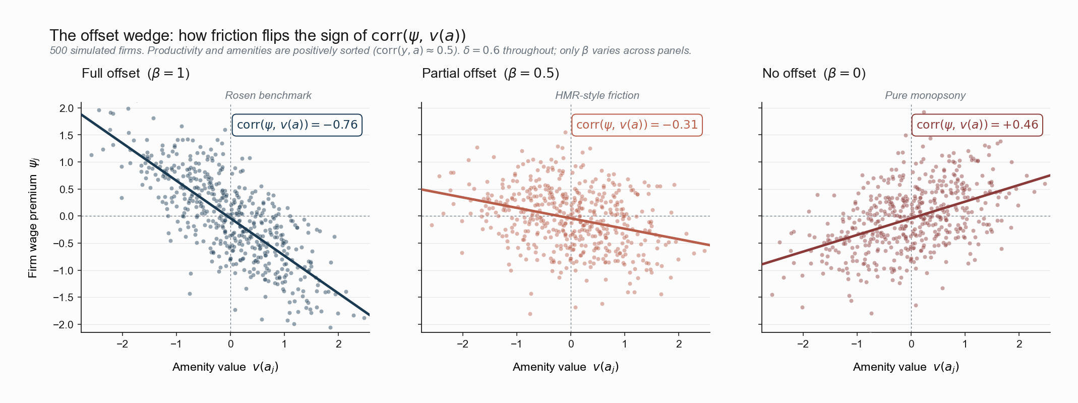
The figure below makes this concrete. We simulate 500 firms with $\mathrm{corr}(y, a) \approx 0.5$, hold $\delta$ fixed, and vary the offset rate $\beta$.

Reproduce the figure

import numpy as np, matplotlib.pyplot as plt

rng = np.random.default_rng(20260522)
N = 500
y = rng.normal(0.0, 1.0, N)              # firm productivity (latent)
a = 0.5 * y + rng.normal(0.0, 0.75, N)   # amenity, positively sorted with y
eps = rng.normal(0.0, 0.20, N)
delta = 0.6                              # productivity rent passthrough

for beta in (1.0, 0.5, 0.0):
    psi = delta * y - beta * a + eps
    print(beta, np.corrcoef(a, psi)[0, 1])

In the leftmost panel ($\beta=1$, full offset), $\mathrm{corr}(\psi, v(a)) \approx -0.76$. The Rosen prediction holds: cash wages compensate for bad amenities. The middle panel ($\beta=0.5$, partial offset under friction) preserves the sign of the relationship but attenuates it to $-0.31$. The rightmost panel ($\beta = 0$, extreme monopsony) flips the sign to $+0.46$, because now only the productivity channel, which is positively correlated with amenities by construction, remains visible.

Two lessons follow.

First, the sign of the observed correlation between $\psi$ and amenities is a structural diagnostic. A strongly negative correlation is evidence that markets approximate Rosen’s frictionless benchmark. A near-zero or positive correlation is evidence of either substantial monopsony or a strong productivity-amenity sorting (and probably both).

Second, the magnitude of $\psi_j$ is no longer a clean measure of firm “quality” in any of these worlds. In the full-offset world, low $\psi$ means good amenities. In the no-offset world, high $\psi$ comes bundled with good amenities. Reading $\psi_j$ literally as a firm pay premium misses two thirds of the story.

Sorkin’s Trick: Watch Where People Move, Not What They Get Paid

If wages can be misleading about how good a job is, what can we use instead? In Search and Matching 3 we introduced Sorkin’s (2018) revealed-preference approach as a method for ranking firms. Here, that ranking has a deeper structural meaning.

The key observation is that workers’ mobility decisions, unlike their wages, are driven by total compensation $\phi_j = \psi_j + v(a_j)$, not by the cash wage $\psi_j$ alone. If workers systematically leave firm $j$ for firm $k$ but not vice versa, then revealed preference says $\phi_k > \phi_j$, even if $\psi_k < \psi_j$.

Think of it this way. If everyone you know who works at the Seattle tech firm is quietly applying to the Columbus university, but no one is going the other way, you have an answer about which job is actually better to hold, regardless of which one’s cash wage is higher. Workers vote with their feet, and their feet observe the total package, not just the cash.

This gives a two-equation identification:

Wage-level data identify $\psi_j$.
Poaching-flow data identify $\phi_j$ (up to scale, via the PageRank-like algorithm in Sorkin’s paper).

The amenity value is then identified residually: \[ v(a_j) \;=\; \phi_j \;-\; \psi_j. \]

Sorkin’s headline finding is that approximately two thirds of the variance of firm value $\phi_j$ comes from non-wage characteristics, that is, from $v(a_j)$ rather than from $\psi_j$. Whatever workers are sorting on, it is mostly not the cash wage. This is a striking number. It says that if you ranked firms by what workers actually choose to work at, and ranked them again by the wage premium they pay, the two rankings would disagree on most of what makes a firm a good place to work.

Lamadon, Mogstad, and Setzler (2022) embed this insight in a structural model of imperfect competition that decomposes firm effects into rent-sharing and amenity components. Taber and Vejlin (2020) push further by combining the revealed-preference logic with Roy-style selection on comparative advantage. Across these papers, the recurrent finding is that amenities are first-order, not residual, and that ignoring them gives misleading welfare conclusions about firm-driven wage inequality.

What the Firm Premium Really Measures

We can now stitch the three readings together into a single decomposition. Up to a worker-specific scale, the AKM firm effect is, in any structural model with productivity, rent, and amenities, of the form \[ \psi_j \;=\; \underbrace{\delta\, y_j}_{\text{productivity rent}} \;+\; \underbrace{r_j}_{\text{posted-wage rent}} \;-\; \underbrace{\beta\, v(a_j)}_{\text{amenity offset}} \;+\; \varepsilon_j . \]

Three forces, two with positive sign and one with negative, are all reduced to a single estimated parameter. The consequences are large.

Inequality decompositions that read $\mathrm{Var}(\psi_j)$ as “firm-driven inequality” overstate it whenever firms vary in $a_j$ at all. The variance of $\phi_j$, not $\psi_j$, is the welfare-relevant object.
Rent-sharing estimates that read $\mathrm{Cov}(\psi_j, \pi_j)$ as evidence of profit sharing can conflate amenity differences with genuine rent transmission.
Sorting estimates $\mathrm{Cov}(\theta_i, \psi_j)$ can be biased in either direction depending on whether high-ability workers also sort on amenities that depress $\psi_j$.

The robust path forward, taken by Sorkin, by LMS, and by the recent structural literature, is to refuse to read $\psi_j$ as a single economic object and instead identify its components separately. The two extra equations one needs come from revealed-preference flows and from variation in amenity provision.

The Handoff: The Most Policy-Relevant Amenity

The compensating-differentials literature traditionally focuses on amenities that are easy to measure but small in dollar terms: commute time, schedule flexibility, on-site amenities. The single largest non-wage amenity in the American labor market, by an order of magnitude, is employer-sponsored health insurance. For a middle-aged worker with a family, $v(a_j)$ from health coverage alone can plausibly run into five-digit dollar values per year. The Columbus offer in the kitchen-table example was already mostly about health insurance, even if we did not name it as such.

It is also the amenity for which all three of Rosen’s frictionless conditions fail simultaneously. The tax exclusion of employer premiums creates a fiscal wedge that distorts the relative price of cash and in-kind compensation. The employer pool generates an information rent that the individual insurance market cannot offer. And the non-portability of coverage across employers creates a search friction with no analogue in the standard amenity literature. A worker who leaves a firm loses not just the wage but the pool.

In the next series we develop the demand and supply sides of insurance markets in their own terms. Then we return here, in the bridge series on job lock, with the formal apparatus to ask the question this note has built toward: how does the most important amenity in the U.S. labor market distort the wage premium $\psi_j$, the sorting $\mathrm{Cov}(\theta_i, \psi_j)$, and the welfare cost of mismatch, all at once?

References

Hwang, H., Mortensen, D. T., & Reed, W. R. (1998). Hedonic Wages and Labor Market Search. Journal of Labor Economics, 16(4), 815–847.

Lamadon, T., Mogstad, M., & Setzler, B. (2022). Imperfect Competition, Compensating Differentials, and Rent Sharing in the U.S. Labor Market. American Economic Review, 112(1), 169–212.

Rosen, S. (1986). The Theory of Equalizing Differences. In O. Ashenfelter & R. Layard (Eds.), Handbook of Labor Economics (Vol. 1, pp. 641–692). Elsevier.

Sorkin, I. (2018). Ranking Firms Using Revealed Preference. The Quarterly Journal of Economics, 133(1), 353–401.

Taber, C., & Vejlin, R. (2020). Estimation of a Roy/Search/Compensating Differential Model of the Labor Market. Econometrica, 88(3), 1031–1069.